Two seconds to a clickable map of your entire workbook

3 Minute Read

Every workbook accumulates tabs. A simple model might have five or six. A budget file shared across a team can have twenty or more, some visible, some hidden, some that nobody quite remembers the purpose of. Finding what you need means clicking along the tab bar, squinting at names, occasionally discovering a tab you had forgotten existed and are now afraid to delete in case it breaks something.

A hyperlinked contents page solves this immediately. The problem is that nobody wants to maintain one manually. The moment you add, rename or hide a tab, it is out of date.

This macro builds it for you in two seconds, every time.

What it produces

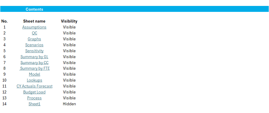
Running the macro creates a new sheet called Contents at the front of the workbook, with three columns:

• No. – tab number in order
• Sheet name – the tab name, hyperlinked so you can click straight to it
• Visibility – whether the tab is Visible, Hidden or VeryHidden

Hidden tabs are included by default, which is the point. A contents page that only shows visible tabs is not a complete map of the workbook.

The sheet gets a colour bar header which can easily be changed to match your company colours by updating the RGB values in the code. Same for the “Contents” font colour.

If you run the macro on a workbook that already has a Contents sheet, it creates Contents2 rather than overwriting. Useful when you are iterating and want to compare versions.

The macro

Paste this into a module. It runs against whichever workbook is active, so it works from your personal macro workbook without modification.

'==============================================================
' Create Simple Contents Page
' Tab number, hyperlinked tab name, visibility indicator
'==============================================================

Option Explicit

Public Sub Create_Contents_Sheet()
    ' Runs against the workbook that is currently active
    CreateContentsSheet ActiveWorkbook, True   ' change to True if we want to include hidden sheets
End Sub

 
' Core routine
Private Sub CreateContentsSheet(ByVal wb As Workbook, Optional ByVal IncludeHidden As Boolean = False)
    Dim contentsName As String
    Dim toc As Worksheet
    Dim ws As Worksheet
    Dim r As Long
    
    If wb Is Nothing Then
        MsgBox "No active workbook detected.", vbExclamation
        Exit Sub
    End If
    
    Application.ScreenUpdating = False
    Application.EnableEvents = False
    Application.Calculation = xlCalculationManual
    
    ' Find next available "Contents", "Contents2", "Contents3", ...
    contentsName = NextAvailableContentsName(wb, "Contents")
    
    ' Create the Contents sheet as the first sheet
    Set toc = wb.Worksheets.Add(Before:=wb.Worksheets(1))
    On Error Resume Next
    toc.name = contentsName
    If Err.Number <> 0 Then
        ' If a naming collision still happens for any reason, append a timestamp
        Err.Clear
        toc.name = contentsName & "_" & Format(Now, "yyyymmdd_hhnnss")
    End If
    On Error GoTo 0
    
    ' Headings
    With toc
        .Range("A4").Value = "No."
        .Range("B4").Value = "Sheet name"
        .Range("C4").Value = "Visibility"
        .Range("A4:C4").Font.Bold = True
    End With
    
    r = 5
    
    ' List sheets and add hyperlinks
    For Each ws In wb.Worksheets
        If ws.name <> toc.name Then
            If IncludeHidden Or ws.Visible = xlSheetVisible Then
                toc.Cells(r, 1).Value = r - 4
                toc.Cells(r, 2).Value = ws.name
                ' Make the name itself clickable (column B)
                AddSheetHyperlink toc.Cells(r, 2), ws.name, "A1"
                ' Also provide an explicit "Go" link in column C
                ' AddSheetHyperlink toc.Cells(r, 3), ws.Name, "A1", "Go"
                toc.Cells(r, 3).Value = SheetVisibilityText(ws)
                r = r + 1
            End If
        End If
    Next ws
    
    ' Tidy up formatting
    With toc
        .Columns("A:D").EntireColumn.AutoFit
        ' Freeze header row
        .Activate
        Range("A:D").HorizontalAlignment = xlCenter
        .Range("A5").Select
        ActiveWindow.FreezePanes = True
        .Range("A1").Select
        .Range("B2").Value = "Contents"
        .Range("B2").Font.Bold = True
        .Range("B2").Font.Color = RGB(255, 255, 255) 'change this to change colour of "Contents"
    
    'Add ColourBar Header
        With Range("A2:M2").Interior
            .Pattern = xlSolid
            .Color = RGB(0, 173, 233)  'change this to change the colour of the colourbar
        End With
    End With
    
    ActiveWindow.DisplayGridlines = False
    Application.Calculation = xlCalculationAutomatic
    Application.EnableEvents = True
    Application.ScreenUpdating = True
    
    MsgBox "Created '" & toc.name & "' with hyperlinks to each sheet.", vbInformation
End Sub
 
' Returns "Contents", "Contents2", "Contents3", ... the first that does not exist
Private Function NextAvailableContentsName(ByVal wb As Workbook, ByVal baseName As String) As String
    Dim n As Long
    Dim candidate As String
    
    candidate = baseName
    n = 1
    Do While SheetExists(wb, candidate)
        n = n + 1
        candidate = baseName & CStr(n)
    Loop
    
    NextAvailableContentsName = candidate
End Function
 
' Check if a sheet name exists
Private Function SheetExists(ByVal wb As Workbook, ByVal sheetName As String) As Boolean
    Dim s As Worksheet
    On Error Resume Next
    Set s = wb.Worksheets(sheetName)
    SheetExists = Not s Is Nothing
    Set s = Nothing
    On Error GoTo 0
End Function
 
' Add a hyperlink to a specific cell on a sheet within the same workbook
Private Sub AddSheetHyperlink(ByVal anchorCell As Range, ByVal targetSheetName As String, _
                              ByVal targetAddress As String, Optional ByVal textToDisplay As String = vbNullString)
    Dim subAddr As String
    subAddr = "'" & targetSheetName & "'!" & targetAddress
    If Len(textToDisplay) = 0 Then
        textToDisplay = targetSheetName
    End If
    
    ' Clear any existing hyperlink on the anchor cell first
    On Error Resume Next
    anchorCell.Hyperlinks.Delete
    On Error GoTo 0
    
    anchorCell.Parent.Hyperlinks.Add Anchor:=anchorCell, Address:="", SubAddress:=subAddr, _
                                     textToDisplay:=textToDisplay
End Sub
 
' Friendly visibility text for the listing
Private Function SheetVisibilityText(ByVal ws As Worksheet) As String
    Select Case ws.Visible
        Case xlSheetVisible:   SheetVisibilityText = "Visible"
        Case xlSheetHidden:    SheetVisibilityText = "Hidden"
        Case xlSheetVeryHidden: SheetVisibilityText = "VeryHidden"
        Case Else:             SheetVisibilityText = "Unknown"
    End Select
End Function

Download the macro as TXT file

Making it yours

The three columns are a starting point. I always add at least one more manually depending on what the workbook is for. On a simple model that might be a brief note of what each tab contains. On a shared workbook it might note who is responsible for completing each section or where the inputs come from. On a more complex model I have used it as a completion checklist so it is obvious at a glance which sections are done. The macro gives you the structure; you decide what additional context is useful.

The colour bar defaults to a bright blue. Two RGB values in the code control the appearance, the header bar colour and the “Contents” font colour. Update those to match your organisation’s colours and it looks like it belongs rather than like something pasted in from outside.

A note on VeryHidden tabs

A tab set to VeryHidden cannot be unhidden through the normal right-click menu, it can only be set and unset via VBA, which means it only exists in macro-enabled workbooks (.xlsm). If you run this macro and see VeryHidden in the visibility column, you now know two things: that tab is deliberately obscured from normal users, and the workbook has VBA capability.

Two seconds to run. Works on any workbook. The only maintenance required is running it again when the tabs change.